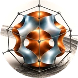
Every band on the phosphor is a lattice plane seen from inside the crystal. This page computes the view.
Pick a crystal and a beam energy. The page follows the electrons: a Monte Carlo of the primary beam in the tilted sample says how many come back out, with what energy, from what depth and in which directions; a many-beam Bloch-wave calculation says how the crystal channels them, once per direction of a symmetry-reduced grid over the sphere (the master pattern); the detector geometry and the Euler angles put that sphere on the phosphor. Turn the crystal, change the energy, switch the energy bins on and off, and compare the dynamical bands with the kinematic band edges drawn over them.
Compute a master pattern to see the detector.
The whole sphere of exit directions in the crystal frame on an equal-area square: the centre is [001], the mid-edges are the [100] and [010] directions, the corners [110]. Move over it to read a direction.
A cut across one band through a general direction, computed exactly (not read off the grid), with the Bragg angle marked. The dark lines of a Kikuchi band sit just outside ±θB; the band between them is brighter than the background because the Bloch wave that channels along the atom planes backscatters more.
The Monte Carlo records every electron that leaves through the surface with more than this energy; the bins divide that range. Each bin gets its own master pattern at the bin's mean energy.
240 × 180 pixels. The pattern centre is the foot of the perpendicular from the beam spot to the screen, measured from the top-left corner. The tilt axis of the sample is horizontal on the screen; the sample normal hits the screen above the pattern centre.
An EBSD pattern is made by electrons that went into the sample, turned around, and came out again through a crystal that steers them. This page computes both halves and puts them together, the way the EMsoft package of De Graef and co-workers does it, entirely in the browser. The first half is a Monte Carlo of the primary beam: single elastic scattering off screened nuclei, continuous slowing down between collisions, in a sample tilted by 70°. For every electron that leaves through the surface it records the energy, the direction of exit and the deepest point of the path, which is the usual stand-in for the depth at which the electron was turned around. The second half is the crystal. By reciprocity, the number of electrons backscattered from the atoms at depth z into a direction d equals the intensity a plane wave would have at those atoms if it came in from that direction and travelled z into the crystal, and that intensity is a many-beam Bloch-wave calculation, the same one that gives the rocking curves on the bend-contour page, with thermal-diffuse absorption. Weighted by the Monte Carlo depth distribution and summed over the depth, it gives one number per direction: the master pattern, the whole sphere of directions in the crystal frame. The sphere is sampled on an equal-area square grid and reduced by the point group of the structure, so a cubic crystal needs one direction in forty-eight. That is thousands of independent many-beam calculations, and on a browser with WebGPU they run on the graphics card as one compute shader; without it they run in JavaScript workers with a coarser grid and fewer beams. The Monte Carlo runs on the graphics card too, one electron history per thread.
The detector is a flat phosphor at a distance L from the beam spot. Every pixel is a direction from the spot; the page turns it into the sample frame (the tilt), then into the crystal frame (the Euler angles), reads the Monte Carlo yield in the first and the master pattern in the second, multiplies by the solid angle of the pixel and draws the result. Because the master pattern is computed once, the orientation, the detector and the choice of energy bins all update at once.
Each Kikuchi band is the trace of one set of lattice planes, brightest between its two edges and darkest just outside them. With kinematic band edges on, the page draws the Kossel cones of the strongest reflections, the directions that make exactly the Bragg angle with the planes, as dashed hyperbolae; the dynamical band sits between them, and the Band profile tab cuts across one band to show where the dark lines fall against θB. The width of a band is 2θB, so the widest bands come from the widest-spaced planes, and all bands widen together at lower voltage. The zone axes, where several bands cross, carry the symmetry of the crystal along that direction. Move the Euler sliders and the whole pattern rotates as a rigid picture of the sphere; the bright-to-dark gradient across the screen does not rotate, because it belongs to the sample, not the crystal: more electrons leave the tilted surface toward the detector side than away from it, and the top of the screen is closer to the beam spot.
The energy bins are the part that is easy to forget. Electrons that lost a quarter of their energy have a longer wavelength and wider bands; their patterns are the same picture at a different scale, and the sum blurs the edges. Switch the energies selector between all bins and the highest bin alone to see how much of the softening of a real pattern is simply the energy spread of the backscattered electrons. The Monte Carlo tab shows the numbers behind the weights: the depth the electrons came from, the energy they kept and the directions they left in.
Two parts add up to the intensity. The channelling part P is the Bloch-wave term: electrons backscattered from atoms while the wave that reached them was still the coherent elastic wave. The incoherent part L counts the electrons that thermal-diffuse scattering had already removed from that wave by the depth in question; the page adds them back as backscattering from the average crystal, a flat background that lowers the contrast without moving anything. With add the incoherent part off you see the channelling term alone, which is what most simulation codes call the master pattern. Flatten the background divides the pattern by a heavily blurred copy of itself, the usual first step in processing a real pattern.
Phrased the way people ask them in EBSD courses, on ResearchGate and in the EMsoft user group. Short answers; the interactive above shows each one.
From the top few tens of nanometres. The Monte Carlo tab shows the depth of the deepest point of every backscattered electron's path: at 20 kV and 70° tilt the median is about 20 nm for copper and nickel, more for light elements, less for heavy ones. Electrons that went deeper mostly do not come back, and the ones that do have lost energy and carry blurred, wider bands. Diffraction contrast needs the coherent elastic wave, which thermal-diffuse scattering removes over a similar depth, so the two limits agree: the pattern is a surface signal, which is why a damaged or oxidised surface layer of a few nanometres ruins it.
Because the source is different. In the TEM the diffusely scattered electrons come from a point-like region and the Kikuchi lines are the excess and deficient lines of a beam being redirected. In EBSD every direction is illuminated by electrons coming from all over the interaction volume, and what varies from direction to direction is how strongly the crystal backscatters electrons travelling that way. By reciprocity that is the channelling condition of a plane wave coming in from that direction. Between the two Bragg conditions of a set of planes the Bloch wave that peaks on the atom planes is strongly excited, and those electrons see the nuclei and backscatter more; just outside the edges the wave that runs between the planes dominates and the yield drops. The profile tab shows both features and marks the Bragg angle, where the transition happens.
The width of a band is twice the Bragg angle, θB = arcsin(λ / 2d). Widely spaced planes (small |g|, like {111} in fcc) give narrow bands; closely spaced planes give wide ones. Halving the voltage stretches the wavelength by about 1.4 and every band with it. The kinematic edges drawn over the pattern use exactly this rule, and the dynamical simulation reproduces the positions to within the width of the dark line. The energy spread of the backscattered electrons is a spread in λ, which is the main reason the edges of a real band are soft.
The channelling yield of a crystal depends only on the direction of the electron in the crystal frame, not on where a detector happens to be. So it is computed once, for every direction on the sphere, and stored on an equal-area square grid: that is the master pattern, the fingerprint of the crystal at one energy. Any detector geometry and any orientation is then a lookup: each pixel of the phosphor is a direction, rotate it into the crystal frame, read the value. The symmetry of the crystal cuts the work by the order of its point group, and the sampling on the square is uniform in solid angle. The same idea is behind dictionary indexing: rather than fitting bands, a measured pattern is compared with patterns looked up from the master for every orientation on a fine grid.
The crystal alone gives the master pattern, but not how many electrons, of what energy, from what depth and in which directions. The Monte Carlo supplies exactly these weights. The depth distribution decides how much dynamical contrast has developed by the time the electrons turn round; the energy distribution decides how much the bands are smeared; the angular distribution is the bright-to-dark gradient across the screen, and the yield sets the absolute level. Change the tilt from 70° to 0° and watch the yield halve, the depth grow and the exit directions turn symmetric.
In principle yes, and this page shows the mechanism. For a crystal with a centre of symmetry the pattern for direction d and for −d are the same and the south square of the master pattern is the north square inverted. Without a centre, the wave coming in from d and from −d see different arrangements of atoms and the two squares differ. The differences are small, a few percent in particular bands, which is why polarity determination by EBSD needs careful pattern matching rather than band positions. Load GaAs or GaN and switch the square selector on the master pattern tab.
The kinematic picture draws lines where the Bragg condition is met and leaves the intensity to a guess. It gets the geometry right, which is all that Hough-transform indexing needs, and nothing else: no band profiles, no intensities, no zone-axis contrast, no dependence on thickness or depth. The dynamical calculation here gives the intensity of every direction from the crystal structure and the physics of channelling and backscattering. It is what pattern-matching methods (dictionary indexing, refinement of the pattern centre, strain from the shift of fine detail) compare experimental patterns against, and it is why those methods work when the bands are too faint for the Hough transform.
Part of it is real: high-order reflections make narrow, faint bands and sharp features at zone axes that a detector with a coarse phosphor and a short exposure averages away. Part of it is what this page leaves out: the point-spread of the phosphor and optics, the noise, the background from other sources, and a surface layer that is not the perfect crystal. Raising the number of beams per direction brings in more of the weak bands and raising the grid resolves them; the readout gives the strength of the weakest beam that was kept.
Not directly. In TKD the electrons that form the pattern go through a thin foil rather than turning round in a bulk sample, so the Monte Carlo geometry is different (a foil, a detector below it) and the depth distribution is the whole foil thickness. The Bloch-wave half is the same physics with a different depth weight. Part 6 of the EBSD series shows the geometry and the resolution argument; the dynamical version is a natural next step for this page.
The master pattern is thousands of independent many-beam calculations, each a matrix exponential with the number of beams cubed in cost, times the number of energy bins. On a graphics card with WebGPU the default settings take a few seconds; in JavaScript workers the page drops to a coarser grid, fewer beams and fewer bins by itself. If it is still slow: fewer energy bins first (the picture barely changes), then the coarser grid, then fewer beams. More electrons in the Monte Carlo only cost time on the graphics card in proportion, and they matter mostly for the smoothness of the angular yield.
The Monte Carlo is Joy's single-scattering model: screened Rutherford elastic scattering with the Joy-Luo stopping power, no secondary electrons, no surface refraction, and a compound treated as a single material with the average Z, A and the density of the cell. Electrons that leave with less than the chosen lowest energy are not recorded. The depth of an electron is taken as the deepest point of its path, and in the Bloch-wave half that depth is measured along the beam direction, as EMsoft does, so that the master pattern is a property of the crystal alone. The Bloch waves use every reflection inside the chosen |g| with the strongest N per direction, ranked by how much amplitude they take from the incident wave and from the strongest beams; there are no Bethe potentials for the rest. For copper at 20 kV the shape of a band profile with 48 beams agrees with 96 beams to 6 percent and 64 beams agree with all 169 reflections inside 15 nm-1 to 3 percent, most of it far from the band; the readout gives the strength of the weakest beam kept. Absorption is the thermal-diffuse absorptive potential in the Einstein model with room-temperature Debye-Waller factors; backscattering is Rutherford, proportional to Z2, with the same Debye-Waller factors. The forward-scattering form of the Bloch-wave equations is used, so beams more than about 10° from the incident direction are coupled slightly too strongly. The graphics-card engine works in single precision and agrees with the double-precision JavaScript engine to better than a part in a thousand of the pattern; the Monte Carlo on the graphics card agrees with the JavaScript one within statistics. There is no detector point-spread, noise or gain, no refraction of the exit direction at the surface, and no surface layer; the crystal frame is the Cartesian frame of the structure library (a along x, b in the xy plane), the Euler angles are Bunge's, and the pattern centre and detector tilt follow the conventions written on the detector card, which are not those of any particular vendor. A CIF you load is treated the same way as a library structure, including the search for its point group.
@misc{tripathy2026ebsdpatternsimulator,
  author = {Tripathy, Manisha},
  title  = {EBSD Pattern Simulator},
  year   = {2026},
  howpublished = {\url{https://untetheredatom.com/ebsd/ebsd-pattern-simulator}},
  note   = {Interactive web tool}
}